I bought a couple of Super Pixie Transceivers when I was studying for my Technician license but only got around to playing with them now. The S-Pixie is a low power, CW transceiver that operates in the 40 meter band at a fixed frequency of 7.023 MHz. The design for the radio has evolved over time and is itself based on older similar designs (see here for some history of similar designs). There is a lot of information on the web about the S-Pixie, for example, one version of a user manual (a longer version of what came with my kit), slideshow describing how the radio works, various reviews, here and here, and plenty of build videos.
At the time I bought the kits I didn’t realize that the radio operated outside the portion of the 40 meter band allocated to Technician license holders (General as well) so I bought some alternate crystals to use. After that I decided to just go ahead and get my Extra license so at this point I’m just using the original crystal that came with the kit.
As planned, I’ve build one kit and am testing it and comparing it to the second kit that I’m building initially on a breadboard. Depending on how my tests go, I might even buy a third kit to allow incremental testing during the build. This would allow directly comparing various portions of the circuit on both the PCB and breadboard, without having loading or interference with the rest of the radio (I had intended this with the first kit, but got carried away one I started soldering).
I have already done a bunch of testing on the first kit build and will compare those results with my experiments with the breadboard build of the second kit. First up, a look at the Pi filter used to connect the antenna to the radio.
Pi Filter – Theoretical Analysis
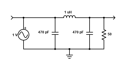
The Pi filter used in the S-Pixie serves mainly as a low pass RF filter. The theoretical cutoff frequency of the filter, f=1/[πsqrt(LC)], is 14.7 MHz given the nominal values of the capacitors and inductor.
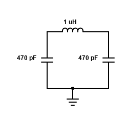
This should provide good attenuation of any harmonics generated by the S-Pixie.
The characteristic impedance of the filter components is close to 50 ohms at their nominal values and the operating frequency of the S-Pixie, 7.023 MHz. A Pi filter is also commonly used to match impedances between two circuits, for example between the RF amplifier and antenna in the S-Pixie. I’m guessing that this was one reason for choosing a Pi filter in older designs, but it isn’t strictly needed anymore (you can tell this as the two capacitors have the same value), meaning the output impedance of the S-Pixie RF amplifier must be close to the assumed impedance of the antenna, 50 ohms. (something I want to look into more later).
Another advantage of selecting a Pi filter over some other low pass filter designs is that the selectivity of a Pi filter can be chosen by selection of the component values. A higher selectivity means a faster fall off above the cutoff frequency. A filter’s Q factor is closely related and deciding on its value is usually a key design decision.
Design Equations
Chapter 5 of the 2023 ARRL Handbook provides the design equations for a Pi network in Figure 5.61 on page 5.30. I couldn’t find a direct online reference to these but they are basically outlined here and here (in the latter, use an center impedance of 25 ohms for our S-Pixie Pi filter).
Using a Q of 1 we get low pass Pi filter capacitor and inductor values of 454 pF and 1.14 uH respectively at 7 MHz. In the ARRL equations, pay particular attention to the sign of X1. It’s negative and effectively causes the second numerator term in X2 to be additive. This confused me at first until I looked at an example in the chapter text which flipped the sign.
Pi Filter – Analysis with Apps
There are a variety of resources available to aid in the design of Pi filters, such as design equations, apps, online calculators, spreadsheets and others. These generally fall into a few categories, such as power supply ripple filtering and impedance matching, and are thus specialized for that purpose. Very few allow you to input the component values and show the filter’s frequency response, though several will provide the cutoff frequency, such as here for example.
The impedance matching methods, of interest to us here, tend to focus on selecting the desired filter Q factor as a key design parameter.
Elsie
Elsie is an electrical filter design and analysis program created by Jim Tonne and available at ARRL Handbook Reference under Software Utilities. The frequency response graph is a nice feature of the program. The program allows you to directly build and analyze your filter network.
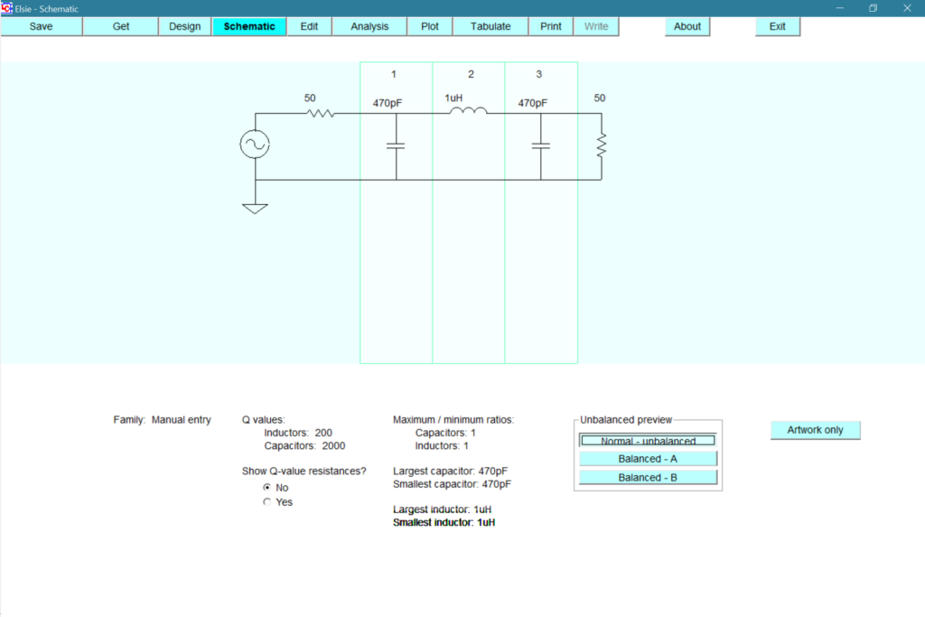
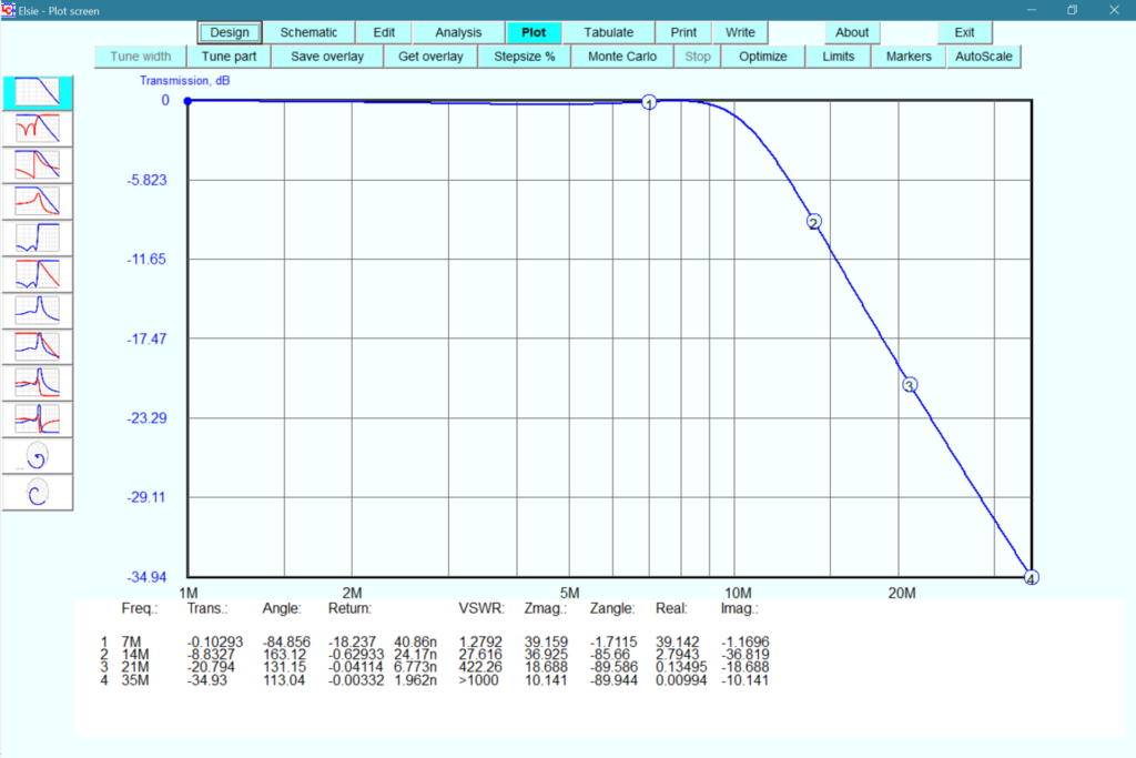
Of note here is the attenuation at 14 MHz, close to the calculated cutoff frequency, is 8.8 dB, well above the commonly used cutoff frequency level of 3 dB which is at about 11.2 MHz for this network from the graph above. The difference may be because the program reflects real world components, but if so I wasn’t able to change the result much by adjusting the inductor and capacitor Q values to more ideal values.
PI-EL
PI-EL is an impedance matching network designer also by Jim Tonne and available in the software download linked above. The program appears to be geared more for impedance matching of tube-based power amplifiers but I think can be adjusted for other circuits. While you can’t directly enter component values in this program, you can tweak the filter Q factor until the calculated component values approximately match the desired values for the desired frequency.
Shown below is a PI-EL design with the Pi section Q set so the S-Pixie Pi filter component values are reflected for 7.023 MHz. Of course this program is designed for a Pi-L network, but here the extra inductor is essentially a short circuit at the frequencies we care about. Interestingly, the resulting Pi section Q factor turns out to be about double the value obtained when using the Pi filter ARRL design equations. I’m not sure of the reason for this, but it’s probably something I’m doing wrong or misinterpreting. The program also provides a frequency response graph.
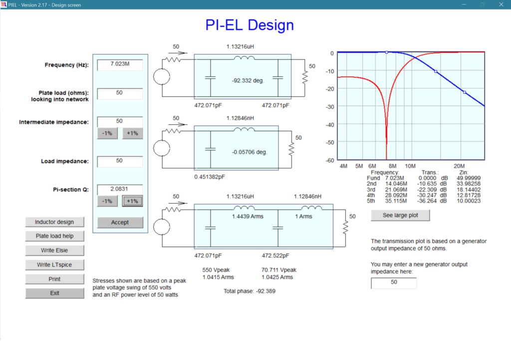
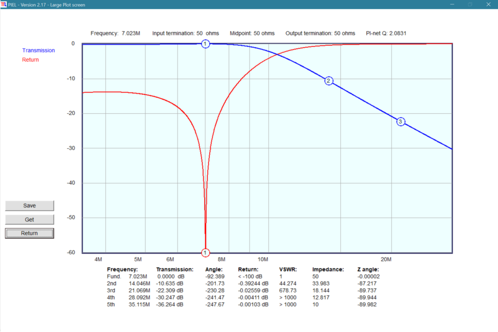
The attenuation values are somewhat higher than those provided by the Elsie program, perhaps reflecting the higher Q factor or extra inductor. Unfortunately, the Elsie program doesn’t provide the circuit Q value.
Online Smith Chart
Will Kelsey has an interesting online Smith Chart tool that allows you to directly build your filter network and see the impact of each component on a Smith chart. A frequency response graph isn’t provided, though a plot of the S11 reflection coefficient is available if you specify a frequency range.
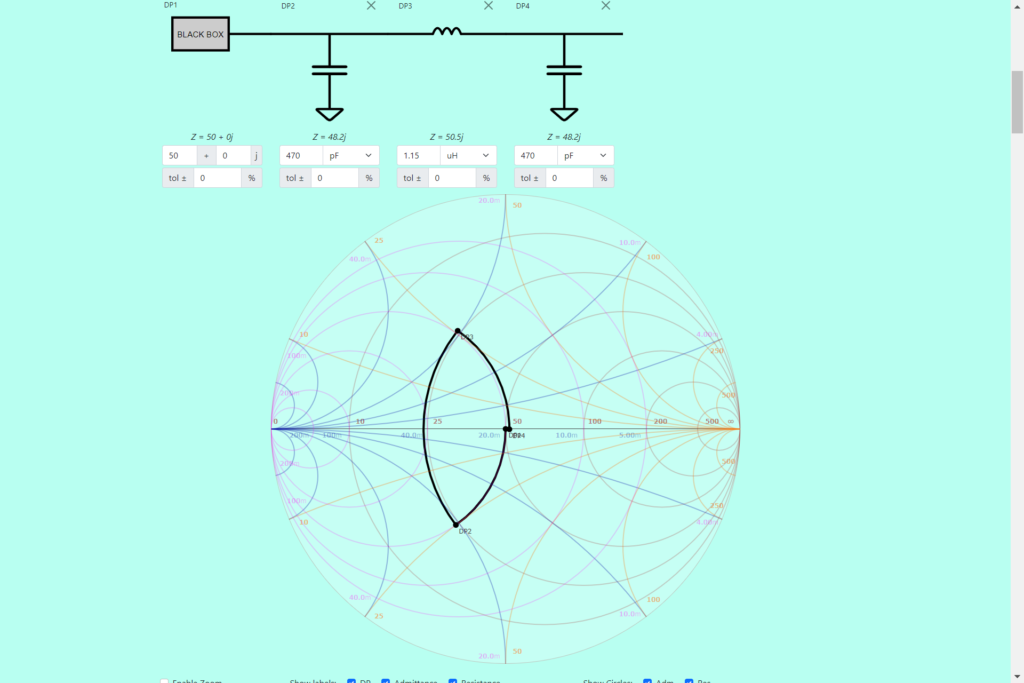
Here I’ve tweaked the inductor value slightly to force a better impedance match.
Pi Filter – Empirical Analysis with AD2 Network Analyzer
I wanted to use my Analog Discovery 2 to examine the frequency response of the filter but you may recall from my last post that I had trouble determining the correct way to connect the AD2 to the DUT (device under test) and interpreting the results.
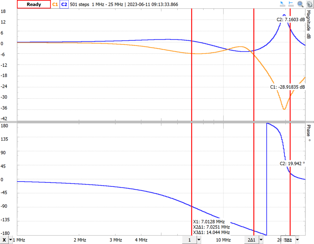
The Network Analyzer provides a tiny, but helpful, schematic diagram for connecting the AD2 to the DUT but that’s the simple part actually. The Pi filter has a clear input and output, unlike the resonant tank circuit in the crystal radio of my last post. If you simply connect the AD2 to the input and output of the Pi filter as specified by the AD2 diagram, you get something like this:
which doesn’t look like the expected frequency response of a Pi filter. Digilent is great in providing a lot of tutorials regarding the use of the AD2, including ones showing the measurement of a few simple circuits, but more examples of circuit analysis would be helpful, including more than simply pointing out the various options available for each instrument used, for example, as within the Network Analyzer.
Part of my problem with interpreting the Network Analyzer plots with the crystal radio experiment was the inductor I was using became capacitive midway through the AM frequency band making much of the network analysis meaningless. That wasn’t the case with the inductor used in the S-Pixie Pi filter. Its inductor showed a normal impedance response through the frequency range of interest. However, I still struggled in obtaining a frequency response plot that I expected or interpreting the ones I got. Eventually, using the examples described in my last post and a little trial and error, I came up with a logical connection scheme that seemed to work and an understanding of what was likely happening in the plot above.
With the AD2 simply connected across the Pi filter as above, the Network Analyzer is showing channel 2, the filter output, at about 20 dB, or a factor of 10 above the reference channel 1 voltage. However, examining channel 1 (not shown above) you get an almost opposite response, that is the channel 1 voltage falls by about a factor of 10 at 7 MHz. Now part of this is due to bandwidth limitations of the AD2, but some of the drop off is likely due to signal reflections from the output back to the input cancelling some of the input signal around 7 MHz. I needed to include a terminating resistor to dampen these reflections.
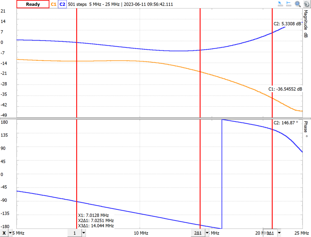
The S-Pixie is designed for a 50 ohm output impedance, so I included a resistor of that value on the output of the Pi filter to simulate the connection to an antenna. Now the AD2 scope and waveform generator channel 1 are connected across the input of the filter (the in arrow in the diagram below) and the scope channel 2 is connected across the output (out arrow).
At mid-range frequencies the resulting plot looked more reasonable (note scale difference). But at higher frequencies, the results still didn’t make much sense.
Now the AD2 does have some limitations at higher frequencies. I was aware of this and it’s one reason I chose to look at the crystal radio previously. AM band frequencies are well within the bandwidth capabilities of the AD2. However, at the frequencies used in the amateur radio HF bands, the AD2 begins experiencing bandwidth limitations, both in its analog inputs and arbitrary waveform generator. You can see some of this in the fall off of the channel 1 signal in the Bode plot above. The AD2 is unable to maintain the level of the 1 volt input sinewave as the frequency increases.
But what’s going on at high frequencies. Is it due to the AD2’s bandwidth limitations or something else. A quick check can be done by using the BNC adapter rather than the flywires used in the measurement above as the BNC adapter has a higher bandwidth.
Well that took care of the strange peak around 20 MHz, but still doesn’t make much sense for a simple low pass filter. Attenuation should continue above 14 MHz, but here we show gain. And why is channel 1 attenuated right from the start?
The latter question is easiest to answer if you’re familiar with the waveform channel connections on the BNC Adapter. The attenuation from the start immediately made me look at the waveform connector termination jumper. The Bode plot above is with the 50 ohm termination jumper set for waveform channel 1. To me this seemed appropriate given I was using a 50 ohm test lead and terminating the filter with a 50 ohm resistor. The BNC reference states, “This enables the user to match the Analog Discovery’s output impedance with either standard 50-ohm test leads or to be directly tied to the lead“. I guess this isn’t appropriate with the Network Analyzer, though it isn’t clear why. Switching the jumper to 0 ohms fixed the early drop off, but not the gain in the response at high frequencies.
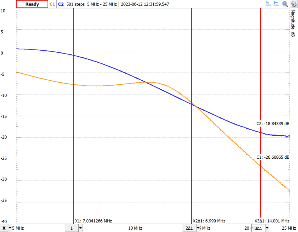
Another thing to check is how I’ve connected the probes to my circuit. This isn’t very critical at lower frequencies, but is at higher frequencies. In the plot above, I had just connected the probes with jumper wires, including the standard probe ground leads. This is problematic at high frequencies and apparently we’re getting there at between 10 and 14 MHz.
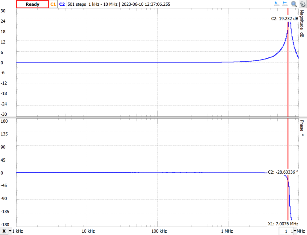
Preparing the Bode plot using the probe tips and grounding springs rather than jumper wires gave better results.
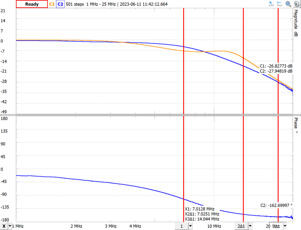
At least the frequency response, channel 2, of the Pi filter declines as frequency increases.
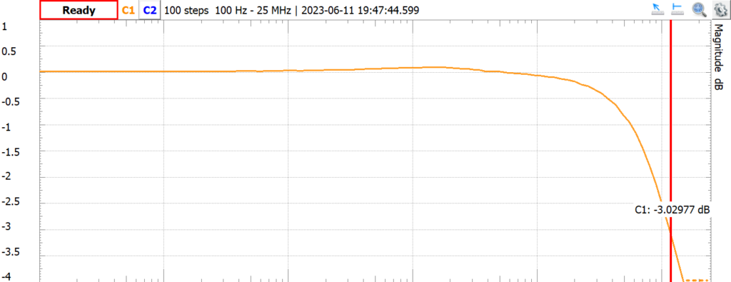
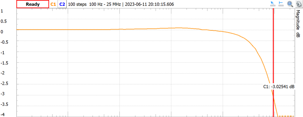
But what is channel 2 actually showing? Has the AD2 made any compensation for the known bandwidth limitations? Digging into the documentation we find that by default, the Network Analyzer shows channel 2 relative to channel 1. So even though the channel 1 voltage drops off due to bandwidth limitations of the AD2, channel 2 should indicate the actual response of the filter.
The actual frequency response of the filter as measured by the AD2 shows a more attenuation than in the analysis programs used above. This could be due to stray capacitance and inductance in the breadboard circuit. I could probably refine the build and use better probes in the measurement, but for me this is close enough for understanding how the circuit is actually performing.
Pi Filter – Empirical Analysis with Oscilloscope and AD2 Waveform Generator
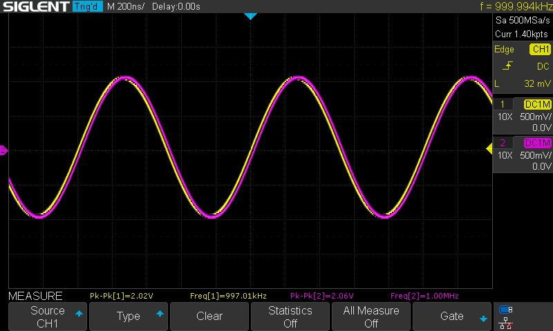
Being somewhat uncertain about the bandwidth limitations of my AD2, I decided to confirm my Network Analyzer findings using my oscilloscope (see the end of this post for an evaluation of my AD2 bandwidth). Since I don’t have a function generator, I decided to use the AD2 waveform generator (the same as used by the Network Analyzer) but manually adjust the signal level as much as possible to maintain a 2 volt peak-to-peak signal. This was possible until somewhat above 14 MHz where I was limited by the AD2 waveform generator voltage limit of +/- 5 volts.
Below are the oscilloscope captures at various frequencies with channel 1 in yellow as the input signal to the Pi filter and maintained at 2 volts peak-to-peak as long as the AD2 was capable and channel 2 in magenta as the corresponding output signal from the filter.
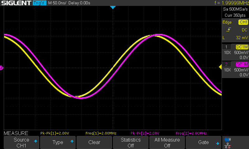
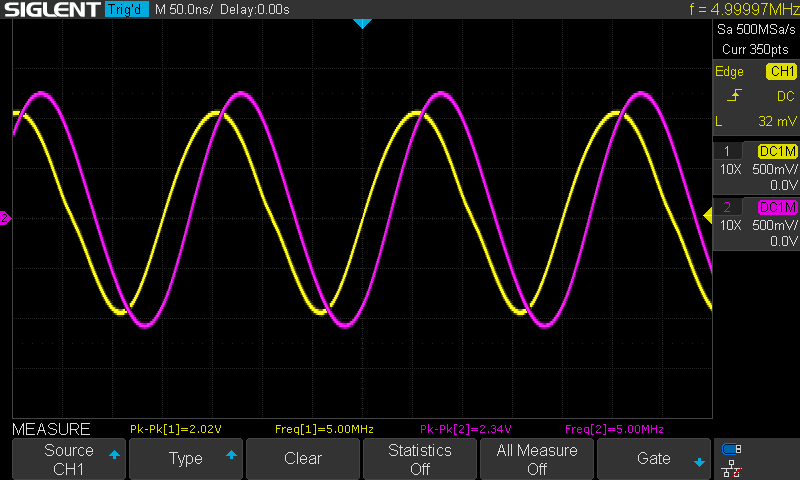
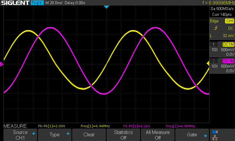
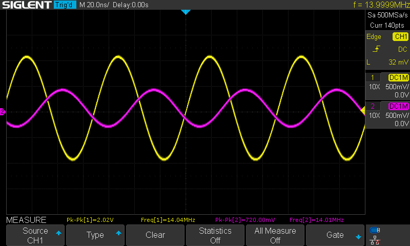
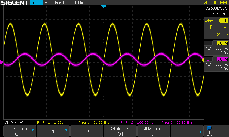
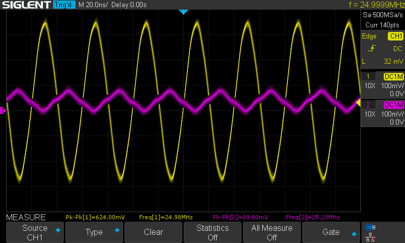
Calculating the gain/attenuation at each frequency:
| Frequency, MHz | Response, dB |
| 1 | 0.17 |
| 2 | 0.34 |
| 5 | 1.23 |
| 7 | 1.06 |
| 14 | -8.96 |
| 21 | -15.67 |
| 25 | -17.01 |
These are closer to the values calculated by the apps than the AD2 Network Analyzer up though about 14 MHz where I was able to maintain a channel 1 signal of 2 volts peak-to-peak. Above that though the attenuation was lower. I was using 200 MHz probes at 10x versus 100 MHz probes at 1x for the Network Analyzer plots, but I don’t think that was an issue here. More likely was just slightly different probe placements and breadboard connections. For example, I went back and ran the Network Analyzer again and got something closer to the values above.
Conclusion
I started my S-Pixie analysis with the output Pi filter because I thought it would be a so,[;e starting place. However, there was a lot more to the analysis than I thought. Next up is the local oscillator. I think it will be easier.
Testing my AD2 Bandwidth
In their AD2 design guide, Digilent summarizes the spectral characteristics of the Scope and Arbitrary Waveform Generator. The spectral characteristics of my AD2 AWG is pretty consistent with these.
I don’t have an external function generator so I can’t independently test the spectral characteristics of my AD2 scope. For now I’ll assume that my scope is in spec given that the AWG is in spec.